Review: “Zoned in the USA: The Origins and Implications of American Land-Use Regulation” (Sonia Hirt)

tl;dr: highly worthwhile book on the international uniqueness of American zoning codes and their cultural underpinnings. 4 out of 5 stars.

This book is an attempt to demonstrate and explain the features of modern zoning codes (and cities) that are almost unique to the United States: the very broad use of exclusively residential zones and exclusively single-family house zones. It combines an extended history of zoning, both internationally and in America, with a comparative study of modern zoning codes and legal regimes surrounding new construction in several countries, most notably England and Germany.

The book is fascinating overall, and highly recommended to any students of cities and/or American history. It is richly detailed and sourced. The perspective is that of an urban planning student from Bulgaria who moved to the US for career reasons and was baffled by the apparent contradictions between the narrative of American individualism and freedom and the very restrictive codes surrounding the built environments in which they lived (which is baffling to this native US citizen as well).

There are many hypotheses that attempt to explain American zoning codes. To name a few: the availability of plenty of cheap land in the US, the predominance of local as opposed to national control over planning and development, the protection of private property values, etc.

However, Hirt feels that these arguments are insufficiently unique to explain the genuine uniqueness of American zoning. The principal thesis of the book is that they are largely the result of a strong cultural undercurrent of agrarian and “frontier” values in the US. As a result, the single-family house on a generous plot was seen as the morally correct dwelling arrangement, and our zoning and legal codes responded to that desire.

The apparent contradiction described above results from the explosion of US cities in the 19th century, and the resulting collision between our preferences for different sorts of “freedoms”: political freedom (in particular the right to use private property without governmental interference) and what she calls “spatial freedom,” which is something like the desire to claim, explore, and patrol the boundaries of a sizable piece of land. It’s not exactly a spoiler to observe that spatial freedom won this rhetorical battle. However, political freedom was appeased in that the new legal structures were simple, scientific, rules-based systems that would treat each property the same and give each property owner the right to development without asking permission within the constraints of the rules, or were advertised as such anyway. And “economic” freedom was appealed to by the universal emphasis on stabilizing and increasing property values.

I did feel that the international comparisons beyond those to Germany and England were a bit overpromised and underdelivered. The sections on each of the other nations discussed (France, Russia, Sweden, Australia, Canada, Japan) amount to capsule histories of a page or two and are not the subject of extended comparisons throughout the rest of the book.

More information about the book is available at Cornell Press.

Thoughts on 51B improvements at Bancroft and College

The intersection of Bancroft Way and College Ave is near the southeast corner of Berkeley’s campus. Caffe Strada, an extremely popular coffee shop, is on the southwest corner, and Freehouse, a relatively new gastropub that seems to be doing pretty well, is to the southeast. To the north is a large plaza which serves as a major entry point to the university. Tons of students walk through this intersection on the way to class from the dorms and apartments further down College Ave.

The intersection also serves the 51B, a major AC Transit bus line with a weekday ridership of over 19,000. The route goes north on College, turns west onto Bancroft at this intersection, and has a stop at the northeast corner. (I’m a regular rider — I take this line probably ~5 times a month to get to and from downtown and the Amtrak station.)

Currently, AC Transit is working with Berkeley to implement improvements along the 51B. This will entail moving bus stops to the far side of intersections, removal of a few stops, bus bulbs, “queue jumps” (removal of a few parking spaces in front of a signalized intersection, so that a bus can move ahead of stopped traffic), new traffic signals at some intersections, roadway widenings, possibly traffic signal priority or special signaling phases for buses. If AC Transit’s proposal is adopted, the line could see improvements of 7 minutes along the line — hugely significant, given that the total route length is only 30 minutes at rush hour.

AC Transit hopes to install a traffic signal at the Bancroft and College intersection to speed buses along. The many pedestrians at this intersection interfere with traffic, and a signal would force pedestrians to wait their turn while cross traffic moves through.

Despite enthusiastically supporting the speed-up plan, I dislike this particular proposal. My sense is that the main problem at Bancroft and College is mostly due to the fact that it’s simply way too large. The crosswalks are 45 to 55 feet from corner to corner, for an intersection which has two traffic lanes in each direction! Pedestrians take 12 to 18 seconds to cross, at typical walking speeds, and buses and cars legally have to wait the entire time that pedestrians are in the crosswalk. Then, because it takes so long for pedestrians to cross, another has generally entered the crosswalk by the time the first has left. It is extremely difficult for vehicles to get a nose in if they’re being polite (as they generally are, to Berkeley’s credit).

The image below shows a simple solution which uses sidewalk extensions to reclaim asphalt for pedestrians, reduce crossing distances to 25-30 feet (7-10 seconds), and generally make it easier for everyone (vehicles included) to cross the intersection.

The shaded regions represent sidewalk extensions that would shrink pedestrian crossing distances to 25 to 30 feet.

The result would be an intersection that is more pleasant, safer, and more efficient for all parties — buses, pedestrians, and cars. (Many of the same considerations apply at Russell and College, another intersection which AC Transit has proposed to put in a traffic signal…)

Best of all, these changes could be implemented as a pilot project for a few hundred bucks with paint and planters. If after a few months it isn’t working, scrap it and start over!

Visualizing population density: New York City

This is the third in a series of posts trying to figure out what various levels of population density look like at street level. Previous posts focused on the Bay Area and Boston (check the former for a mission statement and methodology).

7 people per acre (Munsey Park)

8 (New Rochelle)

11 (Woodmere)

20 (Port Washington)

23 (Jamaica, Queens)

25 (Long Beach)

27 (Jamaica, Queens)

32 (Long Beach)

36 (Glen Oaks, Queens)

44 (Gravesend, Brooklyn)

56 (Jamaica, Queens)

59 (Maspeth, Queens)

73 (Bed-Stuy, Brooklyn)

80 (Harlem, Manhattan)

94 (Bensonhurst, Brooklyn)

110 (Crown Heights, Brooklyn)

113 (Park Slope, Brooklyn)

140 (East Williamsburg, Brooklyn)

183 (Sunset Park, Brooklyn)

 

Not sure what’s going on here — this is a surprisingly high density for townhouses. This is a mostly Asian neighborhood, and so there may be more people per household than in other areas.

184 (West Village, Manhattan)

190 (Chelsea, Manhattan)

199 (Harlem, Manhattan)

200 (Lower East Side, Manhattan)

207 (East Village, Manhattan)

212 (Upper West Side, Manhattan)

320 (Upper East Side, Manhattan)

Visualizing population density: Boston

If you’re interested, you can check out the first post in this series (the San Francisco Bay Area) for a few words about I’m doing this, as well as the methodology I used. With that said, on to the pictures!

3 people per acre (Canton, MA)

 

9 (Brookline, MA)

 

12 (Norwood)

 

 

15 (West Roxbury)

 

23 (Quincy)

30 (West Roxbury)

35 (Dorchester)

50 (Boston)

52 (Brookline)

55 (Boston)

55 (Cambridge)

75 (Boston)

82 (Charlestown)

120 (Boston)

 

This block and the next are at substantially higher densities than comparable San Francisco townhouse neighborhoods. The width of the street accounts for a substantial part of this.

135 (Boston)

175 (Boston)

190 (Boston)

Again, narrow streets contribute substantially to higher densities than San Francisco.

 

Visualizing population density: Bay Area

Population density is frequently described as people (or housing units) per acre. But I don’t have a good feel for how “people per acre” plays out in a real-life context. What does a street with 15 people per acre look like? One with 30 people per acre? A hundred per acre sounds like a lot — is it a lot?

With that in mind, I recently spent quite a bit of time combining a map of census block-level population data in QGIS with the awesome power of Google Street View to get a sense for what population density feels like at street level. I focused on the U.S. because the data was accessible to me, but I’d love to see similar explorations of living arrangements around the world — especially European and Japanese cities.

My strategy was to pick blocks across the metro area that represented a variety of population densities. This was done in a quasi-random way — I tried to distribute the locations around the metro area, and I haven’t picked particularly nice or ugly blocks. I just looked at a map of population densities, picked a likely block, navigated there in Street View, and snapped a screen shot. The population density numbers I quote are the averages of the two adjacent facing blocks.

A caveat is that I focused on streets that were primarily residential, which will have higher population densities than blocks which contain other uses mixed in. On the other hand, residential uses constitute a large majority of the acreage of any city (e.g. 48% for Berkeley), and the figures I quote do include the square footage of the surrounding streets, which constitute 15-25% of the area of a typical city (24% for Berkeley, from the same source).  On net, if you’re interested in bulk population density on a city scale — including shops, schools, offices, parks, etc — you’ll need to deflate these figures by something like 25%.

On to the pictures

1.8 people per acre (Danville):

At the low end, these densities are necessarily imprecise — lot and block sizes aren’t so clear from the air.

3.7 (Danville):

5.8 (Danville):

8 (Danville):

12 (Santa Cruz):

15 (Santa Cruz):

18.5 (Santa Cruz):

25 (Berkeley):

26 (Berkeley):

Both Berkeley and Santa Cruz have a reasonably high fraction of legal or illegal “granny flats” — a separate living unit at the back of the lot. You can see a few in this image.

40 (Santa Cruz):

50 (San Francisco):

Our first townhouse neighborhood is not so high-density: mostly two-story with fairly large backyards

65 (Berkeley):

Individual largish apartment buildings can contribute substantial density.

70 (San Francisco):

Three-story townhouses.

78 (San Francisco):

Slightly smaller lots.

85 (Berkeley):

Fairly large apartment buildings mix with single-family and duplex houses.

125 (San Francisco):

Mostly apartment buildings here.

135 (San Francisco):

Townhouses and apartment buildings. The Bay Area doesn’t get much denser than this.

Safe space for bikes on Shattuck

For the attention-impaired, the short version of my thesis here is that Shattuck Ave, the main street of progressive and bike-friendly Berkeley, CA, is hostile to bicyclists who are not comfortable sharing the road with traffic moving at 30 mph. It is also incredibly wide, which gives us an opportunity to fix this problem. A little ways down the page, I describe a simple and relatively cheap proposal to fix this condition and increase the number of people shopping, socializing, and general moving about in downtown Berkeley. Please read on!

A bit of history

I’m not an expert on the history, so I’ll keep this brief. Shattuck Ave. has long been the Main Street of Berkeley — it’s sufficiently historical that it has a Wikipedia page.

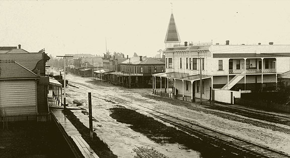
The picture below shows Shattuck in 1892 — follow the link for some interesting local history.

Basically a mud pit with a rail line through it. As Berkeley grew, Shattuck Ave developed commensurately.

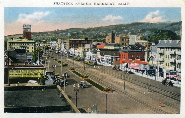
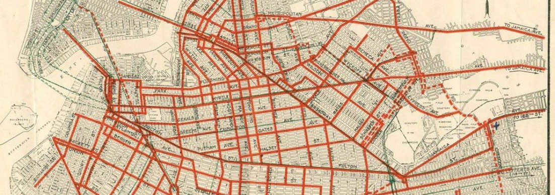
I can’t find a date for this picture, but I would guess late 20s — the 12-story building in the middle is the Wells Fargo Tower, completed in 1925. Talk about wide! There’s space for two entirely separate rail lines — heavy rail and streetcars. The heavy rail hung on until 1941 and the streetcars until 1948.

By the 1970s, like downtowns everywhere, Shattuck was in decline. In conjunction with the opening of the BART in 1973, Berkeley decided that a multi-way boulevard treatment — like Paris! — would revitalize its downtown.

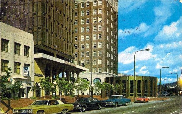
This vivid photochrom image doesn’t actually show the boulevard, but it does show the lovely architecture and automobiles of the time. The area at the bottom of the picture is used as a bus stop instead of parking these days.

The Boulevard

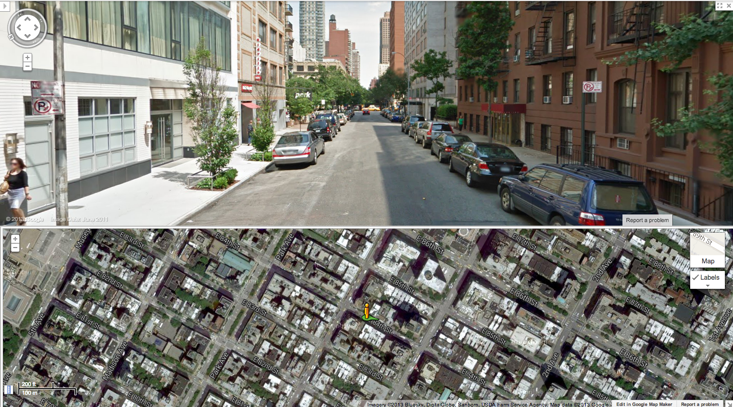
Here’s the street view of a representative block of Shattuck:

You can see how incredibly wide Shattuck is — 4 lanes for moving traffic in the middle, a wide median (which becomes a turning lane at intersections), two access roads, each of which have a moving lane and an angled parking lane, and relatively wide sidewalks on top of that. From building front to building front, the right of way is approximately 160′ wide! At present, 50′ to 60′ of this right of way is for fast cars, 70′ is for slow and stopped cars, and 20′ is for people. (Plus 10′ to 20′ of medians — used for mid-block vigilante picnics further north near Cheeseboard! But not so here.)

Why? A Complete Bicycle Network

Berkeley has a reputation as a bike-friendly city — a reputation which, in the American context, it certainly deserves. The most notable cycling infrastructure is a network of bicycle boulevards. These are principally residential streets which have low traffic volumes and speeds due to traffic diverters, and are indeed the safest way to get to many parts of town by bicycle.

But Berkeley’s bike boulevards as presently implemented have a major drawback: they generally have no commercial development. As a result, one is forced to leave the boulevard network to get to shops and restaurants by bike, and use major streets like Shattuck. Compared to the places one can directly and conveniently access by car, the bicycle network is generally sparse and uninviting. Bicycling is the most efficient mode of urban transportation (in cost, land, and energy) and we have misprioritized our streets.

In this context, it’s distressing that Shattuck is hostile to cyclists. Cars commonly travel upwards of 30 miles an hour, though strictly speaking the speed limit here is 25, and there are red lights at most cross streets (an example of the “hurry up and wait” theory of traffic engineering). As noted above, there are low-speed access lanes mid-block, which the less brave cyclists such as myself tend to use, but this requires re-merging with traffic to cross every intersection. Needless to say, it doesn’t feel safe. Despite this, a respectable number of people bike to and from the downtown Berkeley BART station on a daily basis, and in fact the city has established a Bike Station with secure and cheap/free bicycle parking in a storefront on Shattuck. Berkeley should support these investments with streets that are safe for bicyclists.

A secondary reason is that it would actually be remarkably easy! Shattuck is very wide, at 160′ of right of way, and making a safe space for bicycles without taking away travel lanes or parking spaces is quite straightforward.

A fun aside: residents of a car-optional city have a ton of extra money to spend around town. If you can skip buying a car — at $9122/year ownership costs, by AAA estimates (pdf) — you can afford an extra $157,737 worth of house, on a 4% 30-year mortgage (pretty typical rates these days, though low by historical standards). Safe bike lanes are about dollars and cents.

Safe space for bikes, on the cheap

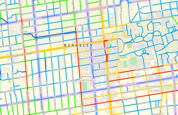
The red line on the following picture marks the nine-block stretch of Shattuck between Allston and Carleton which has the “boulevard” configuration described above, with access lanes and parking on both sides. The project would focus on this area.

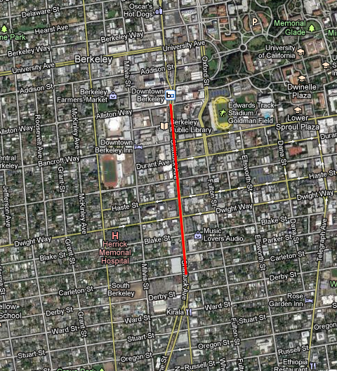
My proposal would simply add curb cuts and bike lanes to connect the access lanes at the intersection. The access lanes would now simply be a throughway for bikes, while still being used by cars accessing the angled parking. In the access lanes, cars are moving sufficiently slowly that sharing space is tenable — this would be plenty comfortable for most people, even (and especially) for those who don’t think of themselves as “cyclists,” and would constitute a massive improvement over the current configuration.

I’ve edited some pictures to give you a sense of what I mean. This one is facing south, at the intersection of Blake and Shattuck:

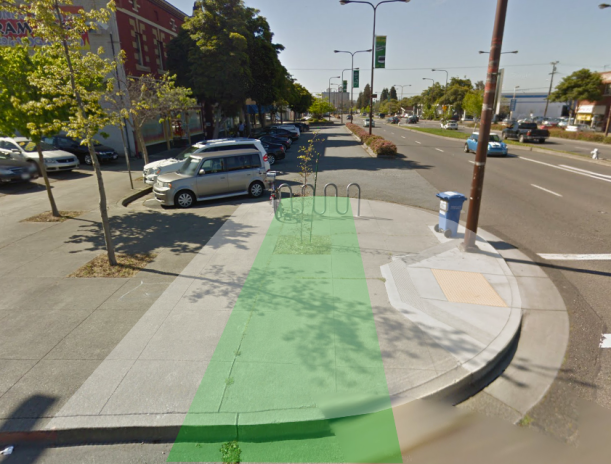
The space that would be repurposed for a bike lane is shaded green, and the space overlaid in white would be lowered to a height of ~1 inch so that the lowered bike lane doesn’t constitute a barrier to pedestrians (see below).

Same intersection, facing north:

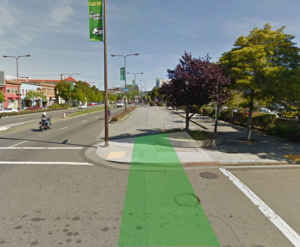
Same as above. Apologies for my meager photo-editing skills!

Obviously the crossings don’t need to be green, but they should be distinctively marked in some way — with some combination of paint and/or pavement — to make them visually obvious to turning drivers.

Implementation-wise, the simplest option would be to simply to cut a path through the pedestrian bulb-outs, so that bicyclists continue through at street level. However, pedestrians should always have the right-of-way before cyclists, and a deep cyclist “trench” would hinder pedestrian movement. I think the main problem is really that the curbs here are too high. I would simply lower the curb for the entire bulb-out (say, from the right edge of the planter leftward in the picture above), so that the bike lane cut-through would only be ~1 inch below the pedestrian space. I ain’t a lawyer, but I imagine that this would also help with ADA-compliance.

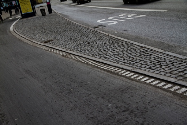
A lowered curb for the entire pedestrian bulb-out would make the cut-through bike lanes much less of an intrusion into the pedestrian realm. The curb/pedestrian island pictured is in Copenhagen.

I see two obstacles to this. The first is fairly minor. The city saw fit — presumably in the last redesign in the early 1970s — to locate massive concrete planters on the southwest and northwest corners of each intersection. As you can see in the picture immediately above, these would need to be removed or relocated. I have no idea how expensive this would be but the planters are pretty imposing in that Brutalist kind of way. (This also serves as a warning about over-designing projects — small is better than big, and fast is better than slow, because if it doesn’t work you can always go in and change it later! Cities need to make more small, experimental investments that potentially have big payoffs.)

The second issue is bigger. There are a total of nine bus stops along this corridor, all of which are recessed from the street, so that buses can pull off to the side for loading/unloading without disrupting traffic. If the bike cut-throughs continued straight on as described above, they would pass directly through the bus loading area. I’ve tried to diagram the problem and my solution for a representative example below, at the corner of Shattuck and Dwight.

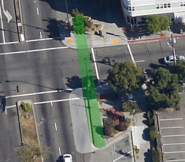
The green area shows where the bike crossing would be. At present, this area passes directly through the bus boarding area. The white area represents an extension of the sidewalk — a bus loading island.

I think the best solution here is to extend the bus stop to be flush with the rest of the access lanes, which would allow plenty of space for the bicycle crossing. This has the downside that a bus stopped for loading and unloading would be blocking a travel lane. However, this is actually a common operating condition for buses in the rest of the world, because this allows the bus to take a straight path, making for a much nicer, smoother, and more reliable ride. (Consider that after pulling over to a stop, buses have to wait for a break in traffic to get moving again!) Furthermore, traffic on this part of Shattuck is not all that severe — most of the delay for cars traveling through this area consists of waiting at red lights. Some political will would need to be mustered, but the benefits for pedestrians, cyclists and public transit outweigh minor delays for car travel.

Costs

How much would this cost? This will be totally uninformed speculation on my part — I have no experience with road or sidewalk construction costs. But maybe a ballpark estimate is better than nothing.

I count 30 bulb-outs along the boulevard-ized part of Shattuck similar to the intersection at Blake pictured above. A very rough estimate of the area we’re reconfiguring on each bulb-out is 1000 sq. ft. The proposal also involves the construction of 9 pedestrian islands at bus boarding locations, at about 1800 sf each. Thus the total square footage is roughly 50,000.

This site estimates that the cost — labor + materials — of replacing an old concrete driveway with stone pavers is about $7/sf. That’s describing a residential use, and it’s probably appropriate to expect that a heavily-used piece of civic infrastructure will cost a bit more — but a city implementing a relatively large construction project can also get economies of scale, so I’ll use $7/sf as a metric, totaling $350,000 for the pavement. Throw in some paint to mark the lanes at intersections and add sharrows in the access lanes, round up a bit, and I think $400,000 is a reasonable expectation for the total cost.

In another post, I’ll describe a slightly more radical proposal for a redesign of the access lanes with a substantial expansion of the pedestrian realm. But for a quick fix on the (relative) cheap, I think this would be a great start. What do you think, Berkeley?

Fact-checking PolitiFact

(I bet nobody’s ever used THAT title for a blog post before…)

A few days ago, the Republican National Committee tweeted “Is it a coincidence that Americans are fleeing tax-and-spend states like CA for states that spend money responsibly? #jobs”. In response, PolitiFact.com published a blog post titled “Are Americans flocking to low-tax states?” in which they half-hearted argued that the data does not show what the RNC claimed.

The research post used a lot of words — it split the states into high- and low-tax groups, and looked at the states within those buckets. We can do better.

Here I’ve used the same data sets that PolitiFact did on net migration and state tax rates. That’s a pretty decent correlation. If you want to play with the data yourself, I’ve uploaded it to Filtergraph, a neat web service that tries to make it easy to work with datasets interactively.

But Why?

Well, who knows. The conservative narrative is that the higher tax rates of states like CA and NY drive workers out of the state. The data is suggestive but doesn’t necessarily prove this. The idea is basically plausible only if you stipulate that state/local governments are providing services that people don’t actually want, or providing desirable services incredibly inefficiently.

(NB: I recently read a paper which pointed out that low-skilled workers are the dominant contribution to the migration rates described above, but that high-skilled workers have very different migration patterns. Specifically, high-skill workers tend to migrate into the largest “knowledge-oriented” metros, such as NYC, San Francisco, or Boston. For skilled labor, productivity and wages are relatively much higher in those areas, but low-skilled workers don’t get enough of a wage bump to make the high cost of living a good trade-off. Unfortunately, I can’t find the paper!)

For fun, I’ve included state-level unemployment in the Filtergraph data set above. Unemployment rates have almost no correlation with either tax rates or out-migration (an R^2 of about 0.09 for each, though Filtergraph won’t automatically calculate best-fit trend lines). So it’s not all that clear that tax rates are closely tied to state economic performance.

Another Narrative: Restrictions on Housing Supply

Why does housing in Manhattan cost so much? The short answer is that supply doesn’t keep up with the demand. Part of this is due to physical restrictions — it’s an island, and building up is somewhat more expensive than building out. But another important contributor is regulatory restrictions. Glaeser et al showed rather elegantly that housing costs on Manhattan south of 125th St. are at least twice as high as the cost of constructing that housing. The authors infer that restrictions on development are contributing significantly to the lack of supply, and thus to the insanely high housing costs. (In 1960 alone, 13,000 new units were permitted in Manhattan, vs. 21,000 for the entire decade of the 90s.)

A less dramatic version of the same story plays out almost everywhere in America where there are people already living, most notably through wildly complicated use-based zoning codes that limit higher-density housing and require too much parking. In most areas, cheap housing can only be built on greenfields at the periphery of the urban area, where there are no neighbors to complain. But because there is no demand for high-density housing in these remote and cheap areas, only detached single-family homes get built. The primary result is auto-oriented sprawl.

Housing costs account for a much higher fraction of the average American’s income than do tax rates. And variation in housing costs is much higher than variation in tax rates. If a large fraction of housing costs in expensive areas is due to regulatory barriers (and not, say, higher local incomes), we might expect low-skilled workers to be driven to cheaper states. I grabbed Census data on median housing costs by state, taking a weighted average of owner-occupied and rental units, and then normalized by median 2009 household income from Wikipedia. (This data is also available on the aforementioned Filtergraph page.)

The evidence isn’t clear. The fit here is statistically weaker than for tax rates. But median housing costs isn’t a perfect proxy for regulation — some states have low housing costs because there’s no demand, not because of a less regulations on development. And low-wage workers don’t get the same salary boost from living in productive metros that high-wage workers typically do, so  median income may not be the appropriate normalization. We really need better data to distinguish between these explanations! In general, though, I’m more sympathetic to the “regulatory tax” narrative, simply because the costs involved can be much larger than the differential tax rates between states.

Cyclist level of comfort in Berkeley

Standard city cycling maps tend to show where there is physical infrastructure: trails, bike lanes, and that sort of thing. For instance, see Berkeley’s map (pdf) of bike lanes and bike boulevards. This is useful information to have, but it falls far short of ideal, because a narrow bike lane on a 35-mph road is a very different thing from a wide lane on a 25-mph residential street. In fact, in many cases, the street with the bike lane will not be the safest or easiest path for cyclists to take.

I’ve made a map which attempts to answer the question: given your personal stress threshold for dealing with traffic, how can you get from here to there on a bike? I was inspired to do this after seeing a similar method applied to Austin, TX in this blog post at the Green Lane Project.

Different colors designate different levels of street comfort and safety for cyclists, from blue (LTS 1, for the kids) to red (LTS 4, for the fearless). Click through for a fully interactive map!

Click on the map for an interactive version, where you can show or hide different street classifications individually.

One fun thing is to turn off the LTS 2, 3, and 4 layers, leaving only the blue routes visible. Berkeley becomes a largely disconnected network of islands, with major streets functioning as barriers. The bike boulevards (shown in purple) alleviate this to some degree, because they usually get signalled intersections.

Read on for much more discussion, including a definition of LTS!

A Taxonomy of Cyclists

The idea guiding this map is a taxonomy of bike riders (and non-riders) developed by Roger Gellar, the bike coordinator for Portland, OR. The basic idea is that there are four types of bike riders. The following descriptions paraphrase heavily from that article.

Gellar estimates that less than 1% of Portland’s population are “Strong and Fearless.” These are the people who ride bicycles in most of the U.S. They are unafraid to use roads with high-speed traffic and narrow shoulders, or to simply take the lane. I think of this group as made up of a combination of people who wear lycra and NYC bike messengers. They’ll ride streets regardless of infrastructure and surface conditions, and being a “bicyclist” is part of their identity. These folks are largely male.

The second group is “Enthused and Confident,” who make up something like 7% of the population. These are the people in Portland who have been attracted to biking as the city has developed its bike network over the last 16 years. They will share the road with traffic but prefers separated infrastructure. This group is the reason why many college towns have relatively high cycling rates: they cycle because it’s a cheap and practical means of transportation, but also because they tend to be overconfident young males who are not so concerned with safety.

A third group, comprising 60% of the population, is “Interested but Concerned.” They wouldn’t mind riding — they probably enjoyed biking when they were a kid, and don’t mind using separated trails. But they’re not confident enough to use city streets, if they even own a bike — they know what will happen if they get hit by a car moving at 35 mph, and they’re understandably uncomfortable to interact with traffic moving at that speed. I don’t know how the 60% figure was arrived at, but it’s worth mentioning that in Amsterdam, close to 40% of trips are made by bicycle (as of 2008) and 85% of the population reports riding a bike in the last week (as of 2003; pdf). Thus 60% of the population may be an underestimate.

Finally, “No Way, No How” makes up about a third of the population. These people just won’t bike, for various personal reasons.

A depiction of the cyclist taxonomy. Clockwise from top left: “Strong and Fearless” (cite), “Enthused and Confident”  (cite), “Interested but Concerned” (cite, which has many other excellent pictures of cycling in Amsterdam) and “No Way, No How” (cite).

Level of Traffic Stress

A report, Low-Stress Bicycling and Network Connectivity (Mekuria et al, 2012) from the Mineta Transportation Institute tries to connect the rider taxonomy above with the physical characteristics of roads. The basic idea is simple: a segment of road with higher speeds and more travel lanes in each direction is less comfortable for cyclists. Conversely, bike lanes can make an stressful road less so.

They break things down into four levels of stress, which correspond to various cyclist types in the taxonomy above. Specifically, LTS 4 is intended to correspond roughly to “Strong and Fearless,” LTS 3 to “Enthused and Confident,” and LTS 2 to “Interested but Concerned.” Finally, LTS 1 is meant to describe roads that an eight-year-old and an eighty-year-old should be able to safely ride.

Stressful intersection crossings contribute to the level of stress of adjacent road segments. Thus, it’s appropriate to think of this map as showing the network connectivity for Berkeley cyclists with different stress thresholds, rather than strictly showing the stress level for each segment.

I won’t go further into the details about the approach. If you’re interested, see the paper; I followed their method pretty closely. A couple of small things:

I made one small modification to their approach. For instance, I decided that a bike lane could never increase the level of stress of a segment. This applies to Channing (east of MLK Way), which has a bike lane which is narrow enough that it would qualify for LTS 2. However, if it didn’t have a bike lane, it would only have LTS 1, because it’s a two-lane residential road with a speed limit of 25 mph. I chose to give it the more generous classification.

On vehicle speeds: all speed limits on streets in Berkeley proper are 25 mph, except for Sacramento St. and San Pablo Ave, which are both 30 mph. (The freeway and frontage roads are also faster, of course). However, this doesn’t fully capture vehicle speeds in practice. I bumped MLK, Ashby, and Dwight (east of MLK) up to 30 mph, consistent with my sense of how fast people are actually going. I also bumped Tunnel Rd. to 35 mph, as it basically serves to feed traffic from Highways 13 and 24 into town, and in my experience people haven’t yet slowed down to the supposed 25 mph speed limit at that point.

Disclaimers and Caveats

Berkeley cyclists, use this map at your own risk! I do think it’s way better than what exists currently, but it’s definitely not perfect.

A useful modification which would bring the scheme a bit more in line with reality would be to account for traffic volumes. A 25-mph road with 250 cars per day is very different from one with 20,000 cars per day, from the perspective of a cyclist. Another idea (albeit a bit orthogonal to this method) would be to account for topography, which I don’t attempt to do at all with this map.

I also didn’t spend too much time making sure that the streets up in the hills are properly coded (basically all the curvy streets to the east and north in the map below). If you’re biking up there, you either know what you’re doing or you’re not too familiar with Berkeley, because they are steep.

More importantly, I think their classifications are somewhat optimistic. I wouldn’t let my (hypothetical) kid ride on parts of the LTS 1 network. And although I’d self-classify as a LTS 3 cyclist, I’m uncomfortable biking on some purportedly LTS 2 streets such as College Ave.

Finally, it’s probably worthwhile to keep Berkeley’s bike boulevards in mind (in purple on the map). They may not be any physically different than neighboring residential streets, but they frequently get some traffic calming and diversion measures. Plus, drivers on those streets are probably more likely to be watching out for bikes.

Data and Tools

This map would have been impossible without the GIS shapefile of the Berkeley street network available at the city’s website here, which includes street widths (a high fraction of which were accurate). It is a bit out of date but still incredibly useful. Thank you, Berkeley!

Existence of bike lanes was taken from both Google Maps and the city’s bicycle network map, available here (pdf). Both were wrong or out-of-date in some small ways. Bike lane widths were measured by hand as accurately as is feasible via the Google Maps Labs “distance calculator” and satellite view. Similarly, whether or not intersections are signalized was confirmed using Google Maps Street View.

The data was analyzed and massaged in QGIS. The map tiles were created via the incredibly useful TileMill, using a base layer from OpenStreetMap, the Wikipedia of map data. I used the Javascript library Leaflet to serve the map.

Needless to say, this would have been a much more difficult project as recently as five years ago. We live in incredible times.

Redevelopment of park-and-ride lot at Ashby BART station

Many transit agencies are reluctant to redevelop park-and-ride lots, even in fairly dense urban areas, for fear of losing ridership. In many but not all cases, this is a valid concern: ridership in the short term would drop if the parking lot was removed. However, this is not the final word, for at least a couple of reasons.

First, park-and-ride lots are typically highly subsidized. In all cases I’m aware of in the BART system, revenues from parking fees don’t even cover the cost of parking lot maintenance, much less the capital costs from the initial construction. At most stations, the standard parking charge is $1 for a full day, and it costs BART a 30% overhead to collect (pdf source). For comparison, the construction cost of a surface parking lot is about $4,000 per space, and BART estimates upkeep costs of $430 annually per space in 2012 dollars (same pdf source). (And if you’re interested, structured parking spaces cost about $20,000 per space in construction costs and $650 in annual maintenance.) The $4,000 capital cost at 3% over its 30-year lifetime annualizes to about $200. Thus, a parking spot that’s occupied 300 days a year makes 300 x $0.70 = $210 in revenue and costs BART $630. BART is paying a pretty hefty cost to “buy” the driver’s ridership.

Second, the park-and-ride lot tends to stifle walkable development in the area. People largely don’t want to live next to big parking lots, and they can make it unpleasant to walk nearby. Thus, the existence of the lot tends to reduce the number of people who can access the station by non-auto modes, in the long term. Given that mass transit requires a sufficient density of jobs and people to even make sense, the utility of the overall system is reduced.

I wrote a paper which analyzes a plausible redevelopment of part of the Ashby BART park-and-ride station, from both a ridership perspective and a cost-benefit perspective. It was originally written for a class last semester, and I’ve modified it only slightly from that version. From the introduction:

I examine BART’s current TOD Policy to understand BART’s various motivations to redevelop its park-and-ride lots (or not). The main body of the paper is a proposal to redevelop 108 parking spaces at southern end of the Ashby BART parking lot (with no provision of replacement parking). I use quite conservative assumptions to estimate that such a development would be fairly profitable, providing a return on investment above 5% for the developer, assuming market conditions comparable to those of other recent developments in Berkeley. The development would also provide a sizeable annual net revenue stream of $475,000 to $640,000 for BART as lessor, relative to current parking upkeep and revenues. Furthermore, the development could actually result in ridership gains, under realistic assumptions. As a result, the development is completely consistent with BART’s stated principles and long-term goals.

The full paper is available here.

Daily rides per bike for major U.S. bike share programs

I used 1.35 as the projected rides/bike/day figure in my Cruzer Bikes proposal, a figure which I grabbed, more-or-less, from Capital Bikeshare’s original projections. It would have been useful to have a list of rides/bike/day for various Bike Share systems across the U.S.

I’ve put together a quick compendium of ridership figures from major bike share programs across the U.S. I’ve included only those for which I could find ridership estimates, and indicated my sources. I couldn’t find 2012 ridership estimates for several, or any ridership estimates at all for several other large-ish systems (Kansas City, Nashville, Chattanooga, Charlotte, and Long Beach, NY… mostly southern cities… hmm. I suspect the figures would be pretty poor if they were available.)

The numbers for bikes and stations are approximations, in that the numbers typically increase over the course of the year. I tried to take some reasonable averages — e.g., if there were 90 bikes for most of the year and 130 in the final couple of months, that’d go down as 100 in the table. I rounded some numbers off. And I tried to figure how many days the system was in service over the given time period, which also required some estimates.

Sorry for the horrendously ugly table. The free version of WordPress doesn’t play nice with tables.

where	launch date	year of stats	nth year	stations	bikes	days	rides	rides/bike/day	source
Miami Beach, FL	Mar-11	2012	2nd	115	1000	365	1,291,000	3.54	source
Washington, DC	Sep-10	jan-june 2012	2nd	187	1500	182	935,000	3.42	source
Boston, MA	Jul-11	2012	2nd	95	1000	239	534,000	2.23	source
Denver, CO	Apr-10	2011	2nd	50	510	217	203,000	1.83	source (pdf)
Minneapolis, MN	Jun-10	2012	3rd	65	700	216	274,000	1.81	source
Madison, WI	May-11	2012	2nd	30	290	258	63,300	0.85	source (pdf)
Boulder, CO	May-11	2011	1st	13	100	220	18,500	0.84	source (pdf)
San Antonio, TX	Mar-11	2011	1st	14	140	275	22,700	0.59	source
Broward County, FL	Dec-11	2012	1st	20	250	180	15,200	0.34	source (pdf)
Chattanooga, TN	Jul-12	jul-dec 2012	1st	30	300	180	12,600	0.23	source

Some notes:

1. Smaller systems don’t do as well (in daily rides per bike). This is pretty understandable — a small system has less network value. If the system doesn’t go where you need to, you can’t use bike share. This will be especially true if you’re trying to compete with the automobile in a relatively spread-out city (e.g., San Antonio and Broward/Ft. Lauderdale).
2. Younger systems don’t do as well. Several of the low-performing systems were in the pilot phase. There is a clear trend of increasing ridership over time within systems, as well. (This is not shown in the chart above, of course.) Bike share systems take some time to be mature and “normal.”

What does this mean for Cruzer Bikes? I suspect that it means 1.35 daily rides per bike is pretty optimistic for the first year, though pretty plausible for the 2nd or 3rd year — though this is likely only true if the system has decent coverage. And I still think 4 (or above) is a reasonable long-term target, keeping in mind that Capital Bikeshare is still growing quickly by this metric.

02/12/13 EDIT: data for the Chattanooga system added to the table. I may try to keep this up-to-date for a little while.